

Several months ago a friend of mine who is a chemical engineer for DuPont, and is involved with sustaining the uptime (increasing the reliability) of production systems, introduced me to a tool.
It is used to help predict when failures of various equipment may occur, regardless of the cause.
Technically this is called multi-cause failures or mixed failure modes.

Bear Hunting
Knowing that I have a mechanical engineering background as well a substantial background in finance, especially regarding portfolio management, he posed to me the question on whether this methodology would work for predicting the next major market correction (or more specifically a bear market).
This proved to be too good an opportunity to learn if this could be another tool in my pocket to at least have a fair chance of projecting a market related “failure” that might be used to make sure my clients are informed of the possibility and its potential timing.
I don’t want to give you the impression that I am becoming a market timer or advocating the practice.
Way of Engineers
However, knowledge utilizing sophisticated tools, especially those combining engineering principles with finance concepts, always intrigue me.
Let me state upfront that engineers are wired differently than most other people. We approach problems from a process perspective and rely heavily on data to base our decisions and designs of processes and equipment.
The prospect of building a tool that could possibly predict the next recession and/or bear market is one of my aspirations.
It is not to time the market. I’m interested in the ability to manage the risk of my clients’ (and my own) portfolios to the low end of their respective risk ranges as the probability of a recession or bear market rises.
Barringer & Associates
My friend sent me an email with several links to Barringer & Associates Inc., which trained them to utilize a tool to improving the reliability of production operations.
One example involved examining the deaths of soldiers in Iraq during the second Gulf War. It easily shows the impact of the surge that started in September 2007 and dramatically reduced the rate of casualties of American soldiers.
Another example was a forecast of the next Space Shuttle failure after Columbia’s, assuming that no changes were made in the process of launching a shuttle (which would be foolish to do).
Finally, there was an example of a situation where a 7.5 mile long (12 KM) section of Houston’s Metrorail light-rail, commuter railroad was considered the world’s most unsafe railroad.
Improvements were put in place as a result of a mid-2004 Texas A&M traffic study and the results was a significant reduction in accidents along that stretch of rail-line.
Market Downturns
After reading these articles, I was curious if the 11 bear markets associated with the recessions we have seen in the post WWII era would follow the same type of pattern and enable a prediction of the next bear market.
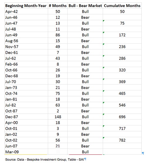
I went in thinking that it would not. I obtained a table from Bespoke Investment Group showing the bull and bear market timeframes for the S&P 500.
I then created a table showing the beginning month and year for each period (as opposed to a daily representation).
I did this since this is the level of detail I work with when making my investment decisions. The table also showed the number of months of the bull market period after which each bear market began and could be considered the first “failure” of the market.
The cumulative months were then calculated. This chart is shown below.
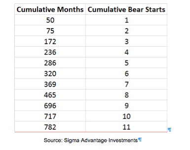
Then, per the process described in the Barringer studies, another table was developed that showed the cumulative months before each market failure (start of a bear market). This is illustrated in the table below.
The final step is to plot the points on a log-log scale. The best fit equation is always a power curve for mixed failure modes.
>Plotting this type of curve on a log-log scale should result in a straight line. The best fit equation is in the form y=λ*xβ where,
· x = Cumulative Time (Months)
· y = Next Bear Market Number (occurrence)
· λ = Coefficient
· β = Power of the power curve
Below is a plot of the data and the best fit curve based on the power curve.
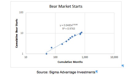
Incredibly, the data had a very good fit! Having an R2 (also called R-squared) in the high 90% range is not often seen, especially with what are considered random events (R2 = 1 is a perfect relationship or fit, 0 is no relationship).
Therefore, utilization of this methodology to predict the next bear market appears to be highly possible.
Next month’s post will evaluate the accuracy of utilizing this methodology to predict the last three bear markets and look at the predictions based on its use for the future.
Photo Credit: KellarW via Flickr Creative Commons


